
Lung Cancer Detection(LCD) from Histopathological Images using Fine-Tuned Deep Neural Network
Received: 14-Jul-2022, Manuscript No. AMHSR-22-69229; Editor assigned: 18-Jul-2022, Pre QC No. AMHSR-22-69229 (PQ); Reviewed: 01-Aug-2022 QC No. AMHSR-22-69229; Revised: 02-Nov-2022, Manuscript No. AMHSR-22-69229 (R); Published: 09-Nov-2022, DOI: 10.54608.annalsmedical.2023.85
Citation: Mishra S, et al.. Lung Cancer Detection (LCD) from Histopathological Images using Fine-Tuned Deep Neural Network. Ann Med Health Sci Res. 2022;12:1-7
This open-access article is distributed under the terms of the Creative Commons Attribution Non-Commercial License (CC BY-NC) (http://creativecommons.org/licenses/by-nc/4.0/), which permits reuse, distribution and reproduction of the article, provided that the original work is properly cited and the reuse is restricted to noncommercial purposes. For commercial reuse, contact reprints@pulsus.com
Abstract
Lung cancer causes hundreds of deaths each year worldwide. The early stage diagnosis and prognosis can significantly reduce the mortality rate. Automatic histopathological image classification plays a keys role in reducing the death due to lung cancer. Now, with the advancement in medical imaging technology, Whole Slide Imaging (WSI) is becoming a routine clinical procedure in pathology. Recently, machine learning and deep learning has shown potential to analysis the pathological images for the early stage cancer prediction such as lung cancer detection. However, training neural networks from scratch requires a large number of labeled images. This is not always feasible, especially with medical imaging data. A promising solution is a transfer learning application on a neural network. In this research paper, transfer learning is applied through ine-tuning the pretrained EffiecientNet-B0 model to detect three different classes of lung cancer. The designed model achieved an accuracy of 99.15%, 99.14%, and 98.67% on the train, test and validation set.
Keywords
Deep learning; Transfer learning; Efficient Net-B0; Fine tuning; Histopathological images
Introduction
It has been observed from the past history that lung cancer is the most common type of cancer found in different age group of people. The causes of this can be smoking, due to exposure to air pollution, radon gas, certain other chemicals, etc. Lung cancer can be divided into two kinds one is small cell lung cancer and other is known as non-small cell lung cancer [1]. About 81% to 85% of lung cancers are NSCLC. There are some main sub types of lung cancer such as squamous cell carcinoma, Adenocarcinoma and large cell carcinoma of NSCLC. These all subtypes derived from different types of lung cells, are grouped as NSCLC. Artificial intelligence is now more popular in the field of health sectors and it has a valuable impact on all aspects of primary care. Early stage detection of any disease can be done with the help of computer vision in the field of medical imaging so that patient can be treated in time and the illness can be cured more simply. There has been eminent research on the usage of artificial Intelligence in the medical domain task such as brain tumor detection, cancer detection from X-Rays, CT scans, pathology images, etc. In this paper, we detect lung cancer from histopathology images with greater accuracy using the transfer learning technique which is applied through fine tuning a pre-trained model. The flow of the paper is as follows. Previous work on the detection of lung cancer is described in section II. The dataset has been discussed in section III. The proposed methodology, preprocessing steps, model architecture, and training has been discussed in section IV. Results are represented in section V. The conclusions of the work done are explained in section VI.
Preliminaries
There are various ways to detect lung cancer using different machine learning and deep learning techniques on several different datasets. Various studies on lung cancer detection has been done by researchers on different datasets. The below is brief descriptions of the research work discussed in papers based on lung cancer detection using different techniques are explained below: Different results have produced from UCI machine learning repository and data world for each classifier for the detection of lung cancer. The results were implemented using DT, LR, NB, and SVM classifiers. Out of all the classifiers It has been shown that SVM performed well on the dataset [2,3]. In this paper the author experimented using deep neural network and auto encoder for lung cancer detection on the Lung Image Database Consortium image collection (LIDC-IDRI) [4]. They were able to achieve the accuracy of 79%, 81%, and 79%, respectively [5]. A method of assembling different combination deep residual network and a classifier on Lung Image Database Consortium image collection (LIDC-IDRI) was proposed, they were able to achieve an accuracy of 84% using Random Forest, an ensemble of U-Net, XGBoost and ResNet [6]. The authors of this paper proposed CNN architectures for lung cancer detection using whole side histopathology images. They used VGG and reset. The outputs of VGG and ResNet were compared using the Receiver Operating Characteristic (ROC) plot. VGG16 model achieved 75.41% patch level accuracy and rested obtained 72.05% of patch level accuracy [7]. In this paper, the authors implemented a CNN network on the LC25000 [8]. The authors used CNN model to classify 3 different classes of lung cancer using lung and colon histopathological image dataset The CNN model developed was able to achieve 96.11 and 97.2% of training and validation accuracy respectively.
Description of dataset
In this work, LC25000 dataset is used. It is a dataset that includes 25000 color images with five classes of 5000 images each. It has 3 types of lung cancer and 2 types of colon cancer. This dataset deals with histopathological images. All images are 768 × 768 pixels in size with JPEG file format. Histopathology refers to the microscopic examination of tissue in order to study the manifestations of disease. Specifically, in clinical medicine, histopathology refers to the examination of a biopsy or surgical specimen by a pathologist, after the specimen has been processed and histological sections have been placed onto glass slides. Histopathologists provide a diagnostic service for cancer; they handle the cells and tissues removed from suspicious ‘lumps and bumps’ identify the nature of the abnormality and, if malignant, provide information to the clinician about the type of cancer, its grade and, for some cancers, its responsiveness to certain treatments. With the help of sophisticated imaging techniques, biopsy tissue can now be obtained from previously inaccessible sites such as the pancreas or retro peritoneum. Tissue is then processed, usually overnight, before being examined under a microscope (Figure 1).

Figure 1: Histopathological Images.
The following are five classes in the dataset, each with 5,000 images:
• Lung benign tissue
• Lung adenocarcinoma
• Lung squamous cell carcinoma
• Colon adenocarcinoma
• Colon benign tissue
• Histopathology
Lung benign tissue: The following points describe the lung benign tissues. Some sample images are shown in Figure 2.
• A benign lung tumor is an abnormal growth of tissue that serves no purpose and is found not to be cancerous.
• Benign lung tumors may grow from many different structures in the lung.
• Determining whether a nodule is a benign tumor or an early stage of cancer is very important.
• Its growth rate is very slow and stops after sometime.
• It does not spread to other parts of the body.

Figure 2: Sample images of lung benign tissue.
Lung adenocarcinoma: The following points describe the lung adenocarcinoma. Some sample images are shown in Figure 3.

Figure 3: Sample images of lung adenocarcinoma.
• It is the most common lung cancer found.
• This type of lung cancer occurs mainly in people who currently smoke or formerly smoked.
• But it is also the most common type of lung cancer seen in people who don't smoke.
• It is more common in women than in men, and it is more likely to occur in younger people than other types of lung cancer.
• Adenocarcinoma is usually found in the outer parts of the lung and is more likely to be found before it has spread.
• Risk of death is low but it is also the leading cause of cancer death.
• Lung Squamous Cell Carcinoma (SSC): The following points describe the lung squamous cell carcinoma. Some sample images are shown in Figure 4.

Figure 4: Sample images of lung squamous cell carcinoma.
• Squamous cell carcinoma is a malignant type of lung cancer.
• It usually begins growing in the cells lining the bronchi.
• Over time, cancer can spread by invading nearby lymph nodes and organs and traveling through the blood (metastasizing) to other parts of the body.
• It has a strong connection with smoking history.
• Risk of death is also high.
• Other risk factors for SCC include-Age, family history and exposure to second-hand smoke.
Materials and Methods
The methodology of this research is based on Efficient Net- B0 [9] model which is pre trained on image net and finetuned it replacing the last output layer with a stack of a few linear and dropout layers and trained the model by freezing the all the layers except the additional layers with the 70% of the total data and the remaining data was used for evaluation. The model was able to produce more efficiency and accuracy than previous ConvNets. Back before using deep learning models we often used three different sets (Figure 5).
• A train set is used for training the model.
• A validation set that is used to evaluate the model during the training process.
• A test set that is used to evaluate the final model accuracy before deployment.
The step by step procedure of this work is mentioned below:
• Input the images from LC25000 dataset.
• Pre-processing is to be done on the images like resizing of images etc.
• Train the Efficient Net B0 model using transfer learning and fine tuning on the validation set.
• Apply the ADAM optimizer and loss function to the model
• Evaluate the performance of the model.
• Improve the results by changing the hyper parameters.
• After that evaluate model on test set.

Figure 5: Structure of proposed model.
Data preparation
Data pre-processing is pivotal for the classification of histopathological images. The dataset contains quite a large image, while the convolution neural network is usually designed to accept much smaller inputs. Therefore, the images were resized from 768 × 768 to 224 × 224. We have divided the dataset for training, testing and validation in the ratio of 7:2:1. The classes were equally represented. Data splitting into training, validation and testing is shown in Figures 6 and 7.

Figure 6: Splitting of dataset.

Figure 7: Dataset distribution for each class.
The following pre-processing techniques were applied to the data
Image resizing: Resizing images is an important preprocessing step in computer vision. Principally, our machine learning models train faster on smaller images. Moreover, many deep learning model architectures require that our images are the same size and our raw collected images may vary in size. Since neural networks receive inputs of the same size, all images need to be resized to a fixed size before inputting them to the CNN. The original size of the image in the dataset is 768 × 768 which is quite large. The images are resized to 224 × 224 using computer vision as it helps to train the model faster and is computationally less expensive.
Dataset splitting: One of the golden rules in machine learning is to split your dataset into train, validation, and test set. The reason we do that is very simple. If we would not split the data into different sets the model would be evaluated on the same data, it has seen. During training, we therefore could run into problems such as over fitting without even knowing it.
Fine tune
We used Efficient Net-B0 model. This model is pre-trained on ImageNet and fine-tuned it by replacing the last layer with a sequence of a few linear and dropout layers. Here, we have used 2 dense layers with ReLu activation function. ReLu (f(x)=max (0, x)) with a dropout layer having dropout rate of 0.2. To avoid over fitting of the model dropout should be used. After each dense layer were added and a final output dense layer was attached.
Model training and testing strategy
For training of model we used adaptive moment estimation (Adam) optimizer and categorical cross entropy loss function was used to calculate the loss of the model. The model was trained with a batch size of 32 for 15 epochs. The model was validated on the validation set after every epoch and the model weights were saved if there was an improvement in the validation loss so that the model with the lowest validation loss was saved. PyTorch package is used for implementation. Publicly available pre-trained Efficient Net-B0 model was utilized [9,10]. The model was trained and tested on Kaggle kernels which provide 12 GB RAM and a 16 GB Nvidia P100 graphics processing unit. Table 1 shows the details of specification used for implementation.
| Table 1: Details of specification used. | |
|---|---|
| Model | Efficient Net-B0 |
| Used Software | Python |
| Image Size | 224 × 224 |
| Batch Size | 32 |
| Learning Rate | 1.00E-03 |
| Epochs | 15 |
| Additional Layers | 5 |
| Dropout Rate | 0.2 |
| Optimizer | Adam |
| Loss Function | Cross Entropy Loss |
Optimization methods
The main purpose of optimization methods is to update the weights at every batch to find global minima. In the Stochastic Gradient Descent (SGD) method [11], the weights update is performed for each training set. Because of this reason, it tries to achieve the goal as early as possible time. The formulation of SGD optimization is shown in equation (1). Here, θ the weight vector to be updated, α is the learning coefficient and ∇θ (θ) is the cost function.

Stochastic Gradient Descent with warm Restarts (SGDR) is a variant of teach rate scheduler, which gradually decreases the Learning Rate (LR) in defined cycles while model is training. SGDR uses cosine annealing, which decreases the learning rate in the form of half a cosine curve. Here ηi the learning rate at time step t (incremented each mini-batch), ηimax and ηimax define the range of desired learning rates, TCurrent represents the number of epochs since the last restart (this value is calculated at every iteration and thus can take on fractional values), and Ti defines the number of epochs in a cycle [12]. The main formula of the SGDR method is shown in equation (2). The arguments used in the SGDR method are:
• Minimum LR-Maximum LR: The lower and upper bound of the learning rate range for the experiment.
• Steps per epoch: Number of mini-batches in the dataset. Calculated as (epoch size/batch size).
• LR decay: Reduce the maximum LR after the completion of each cycle.
• Cycle length: Initial number of epochs in a cycle.
• Multiplication factor: Scale epochs to restart after each full cycle completion.
The ADAM method is one of the methods that update the learning coefficient in each batch [13,14]. It adopts parameter learning rates based on the average first moment in RMS Prop. It also uses the average of the second moments of the slopes. This method is designed with the advantages of the RMS Prop method. In other words, this is one of the optimization methods that update the learning coefficient in each batch. The most important feature of the ADAM method is that it adjusts the learning rate of the weight parameters by estimating the first and second gradient moments in the model network. The ADAM uses the exponential moving averages that are evaluated on a valid mini-batch event and calculated on the gradient. The past gradient (mt) and past square gradient (Vt) averages are calculated according to equation (3) and equation (4). β is the variable used to calculate hyper parameters and usually takes values between 0.9 and 0.999 [15].
Machine learning method
The Soft ax activation function is often used in the final layer of a neural network based classifier. Such networks are commonly trained under a log loss or cross-entropy regime, giving a non-linear variant of multinomial logistic regression. The Soft ax method is generally used in classification processes where the classification label can take more value. Soft ax was used as the activation function in the last layer of the t model. A Multi-Layer Perceptron (MLP) is a forwardclass artificial neural network. An MLP consists of at least three-node layers: an input layer, a hidden layer, and an output layer. The MLP employs a supervised learning technique called training for back propagation. Multiple layers and non-linear activation distinguish MLP from a linear sensor and MLP separates data that cannot be separated linearly.
Evaluation criteria
In order to measure the performance of the developed model accuracy (Acc), precision (Pre), recall (Rec), f1-score metrics are computed along with the confusion matrix. The formulations of the metrics are described as follows in equations (5), (6), (7) and (8).
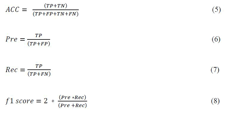
Where, True Positive (TP) represents the number of images classified as cancerous lung whereas True Negative (TN) represents the number of normal lung images classified as lung. Also, False Positive (FP) represents the number of normal lung images incorrectly classified as cancerous lung while False Negative (FN) represents the number of cancerous lung images misclassified as normal lung.
Results and Discussion
The best model weights were saved at the 14th epoch as the model achieved the least validation loss at that epoch. The model achieved 99.15%, 99.14%, and 98.67% accuracy on train, validation, and test sets, respectively (Table 2).
| Table 2: Model accuracy. | |||
|---|---|---|---|
| Model | Training Acc (%) | Validation Acc (%) | Test Acc (%) |
| EfficientNet-B0 | 99.15 | 99.14 | 98.67 |
Figure 8 shows the plot between model accuracy and training accuracy with respect to number of epochs. Figure 9 shows the plot of training loss and validation loss with respect to number of epochs.

Figure 8: Model Training and validation accuracy vs. epoch.

Figure 9: Model training and validation loss vs. epochs.
Table 3 represents accuracy, precision, recall and f1-score for custom CNN Model and efficientNet-B0 Model on test set (Figure 10).
| Table 3: Accuracy, precision, recall, and f1-score of model on test set. | ||||
|---|---|---|---|---|
| Model | Category of Lung Cancer | Precision (%) | Recall (%) | F1-Score (%) |
| Custom CNN model | Adenocarcinoma | 95 | 97 | 96 |
| Benign tissue | 100 | 100 | 100 | |
| Squamous cell carcinoma | 97 | 95 | 96 | |
| Efficient Net-B0 | Adenocarcinoma | 99 | 97 | 98 |
| Benign tissue | 100 | 100 | 100 | |
| Squamous Cell Carcinoma | 97 | 99 | 98 | |

Figure 10: Confusion matrix of proposed model with different image categories for validation and test dataset.
Categories of histopathological images for custom CNN Model and efficient Net-B0 model on test set. The formula for calculating the specified metric is described in section IVD. The confusion matrix shown in and depicts the actual label vs. the predicted label of the images for the validation and test data respectively for a particular labeled category.
Conclusion
In this paper, we make an attempt to detect lung cancer from histopathological images using the transfer learning technique which was employed in the form of fine-tuning. The EfficientNet-B0 model was used as a feature extractor which was then extended with a few additional layers to classify the image into three different classes of lung cancer. The model achieved an accuracy (Acc) of 99.15% on the training set, 99.14% on the validation, and 98.67% on the test. Precision (Pre), Recall (Rec), and f1-score were calculated and a confusion matrix plot was plotted to measure the performance of the model.
References
- Radhika PR, Rakhi AS Nair, Veena GA. Comparative Study of Lung Cancer Detection using Machine Learning Algorithms. IEEE International Conference on Electrical, Coimbatore, India, 2019. [Crossref][Googlescholar]
- Sun W, Zheng B, Qian W. Computer aided lung cancer diagnosis with deep learning algorithms. In: SPIE Medical Imaging. Int j opt photonics. 2016;9785:1-8. [Crossref][Googlescholar][Indexed]
- Armato SG. The lung image database consortium (LIDC) and image data-base resource initiative (IDRI): a completed reference database of lung nodules on CT scans. Med Phys. 2011;38:915-931. [Crossref][Googlescholar][Indexed]
- Bhatia S, Sinha Y, Goel L. Lung Cancer Detection: A Deep Learning Approach. Soft Comput. 2019; 817:699-705. [Crossref][Googlescholar][Indexed]
- Sari C, Russo M, Stella M, Sikora M. CNN-based Method for Lung Cancer Detection in Whole Slide Histopathology Images. IEEE Xplore. 2019;19:1-4. [Crossref][Googlescholar]
- Bijaya Kumar Hatuwal, Himal Chand Thapa. Lung Cancer Detection Using Convolutional Neural Network on Histopathological Images. Int J Comput Techno Appl. 2020;68:21-24. [Crossref][Googlescholar]
- Borkowski AA, Bui MM, Thomas LB, Wilson CP, DeLand LA, et al. Lung and Colon Cancer Histopathological Image Dataset. Arxiv. 2019;1:1-2. [Crossref][Googlescholar][Indexed]
- Tan M, Quoc V. Efficientnet: Rethinking model scaling for convolutional neural networks. Arxiv. 2019;97:1-11[Crossref][Googlescholar][Indexed]
- Wilson AC, Roelofs AC, Stern M, Srebro N, Recht B. The marginal value of adaptive gradient methods in machine learning. Mach Learn.170:1-14. [Crossref][Googlescholar][Indexed]
- Ruder S. An overview of gradient descent optimization algorithms. Machine Learning. 2016;2:1-14. [Crossref][Googlescholar]
- Loshchilov F, Hutter SGDR: Stochastic Gradient Descent with Warm Restarts. 2017;1:1-16. [Crossref][Googlescholar][Indexed]
- Shindjalova R, Prodanova K, Svechtarov V. Modeling data for tilted implants in grafted withbio-oss maxillary sinuses using logistic regression, AIP Conf Proc. 2014:1631:58-62.[Crossref][Googlescholar]
- Wibowo A, Wiryawan PW, Nuqoyati NI. Optimization of neural network for cancer microRNA biomarkers classification. J Phys Conf Ser. 2019;1217:1-9. [Crossref][Googlescholar][Indexed]
- Vamplew P, Dazeley R, Foale C. Neurocomputing Softmax exploration strategies for multiobjective reinforcement learning, Neurocomputing. 2017;263:74-86. [Crossref][Googlescholar]
- Choubin B, Khalighi-Sigaroodi S, Malekian A, Kisi A. Multiple linear regression, multi-layer perceptron network and adaptive neuro-fuzzy inference system for forecasting precipitation based on large-scale climate signals. Hydrol Sci J. 2016;61:1001-1009.[Crossref][Googlescholar][Indexed]


 The Annals of Medical and Health Sciences Research is a monthly multidisciplinary medical journal.